Quick Start
Process your first field with XelToFab
Python API
Basic workflow
Load a field, run the pipeline, and save the result:
from xeltofab.io import load_field, save_mesh
from xeltofab.pipeline import process

# Load a 3D scalar field
state = load_field("field.npy")

# Run the full pipeline: preprocess -> extract -> smooth
result = process(state)

# Save the triangle mesh
save_mesh(result, "output.stl")
The save_mesh function supports STL, OBJ, and PLY output formats (determined by file extension). It uses the best_vertices property, which returns Taubin-smoothed vertices when available.
Custom parameters
Configure the pipeline with PipelineParams:
from xeltofab.io import load_field, save_mesh
from xeltofab.pipeline import process
from xeltofab.state import PipelineParams

params = PipelineParams(
    threshold=0.4,
    smooth_sigma=1.5,
    morph_radius=2,
    taubin_iterations=30,
)
state = load_field("field.npy", params=params)
result = process(state)
save_mesh(result, "output.stl")
See the Parameters guide for the full reference.
2D fields
For 2D fields, the pipeline extracts contours instead of a triangle mesh. Use plot_result or plot_comparison to visualize:
from xeltofab.io import load_field
from xeltofab.pipeline import process
from xeltofab.field_plots import plot_comparison

state = load_field("beam_2d.npy")
result = process(state)

fig = plot_comparison(result)
fig.savefig("comparison.png", dpi=150)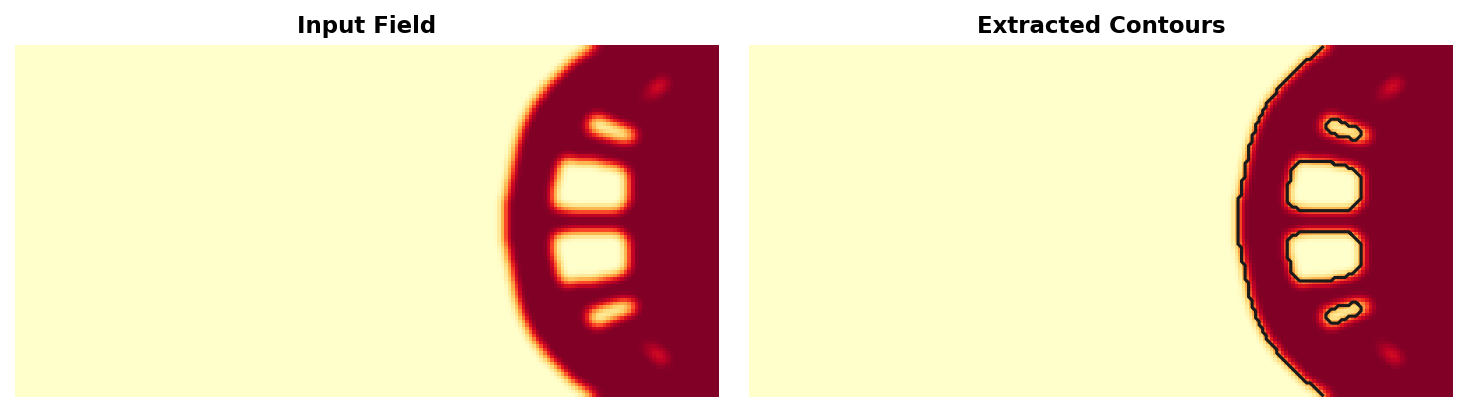
The pipeline automatically detects 2D vs 3D based on the array dimensions. 2D fields produce contour arrays (stored in result.contours), while 3D fields produce triangle meshes (stored in result.vertices and result.faces).
2D → 3D extrusion
When you want a print-ready 3D part from a 2D density or SDF field — rather than contours for plotting — use extrude_2d:
import numpy as np
import xeltofab as xtf

field = np.load("density_2d.npy")
mesh = xtf.extrude_2d(field, thickness=10)
mesh.export("part.stl")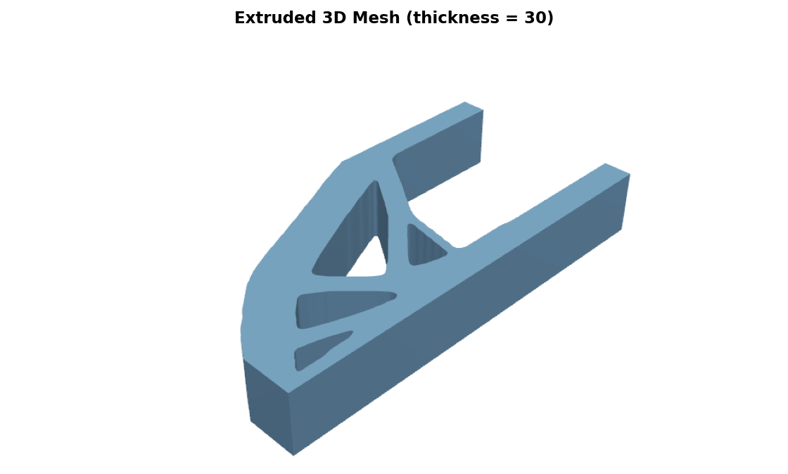
This traces the field with marching squares, triangulates the resulting polygons, and stitches vertical walls into a watertight prism. See the extrude_2d API reference or xtf extrude for the full option set including SDF inputs, pinhole cleanup, and island removal.
SDF fields
For signed distance fields (from neural models like DeepSDF, NITO, or NTopo), set field_type="sdf":
from xeltofab.io import load_field, save_mesh
from xeltofab.pipeline import process
from xeltofab.state import PipelineParams

params = PipelineParams(field_type="sdf")
state = load_field("sdf_field.npy", params=params)
result = process(state)
save_mesh(result, "output.stl")
SDF mode automatically enables direct extraction (skipping preprocessing) and sets the extraction level to 0.0 (the zero level set). See Field Types for details.
SDF functions (neural models)
For SDF functions (neural networks, analytical formulas, or any callable), use process_from_sdf instead of loading a grid:
import numpy as np
from xeltofab import process_from_sdf, save_mesh

# Any callable: [N, 3] → [N] signed distances
def my_sdf(points: np.ndarray) -> np.ndarray:
    return np.linalg.norm(points, axis=1) - 1.0  # unit sphere

result = process_from_sdf(my_sdf, bounds=(-2, -2, -2, 2, 2, 2), resolution=64)
save_mesh(result, "sphere.stl")
This evaluates the function on a uniform grid internally, then runs the full pipeline. Works with any SDF source — PyTorch models, ONNX, analytical formulas. See the SDF Functions guide for details.
Adaptive evaluation for large grids
For high-resolution grids or expensive SDF functions, enable octree-accelerated evaluation to skip regions far from the surface:
result = process_from_sdf(
    my_sdf,
    bounds=(-2, -2, -2, 2, 2, 2),
    resolution=256,
    adaptive=True,      # octree: ~O(N²) instead of O(N³) evaluations
)
save_mesh(result, "sphere_hires.stl")
See Uniform vs adaptive for when adaptive evaluation helps.
Feature-preserving smoothing
For meshes with sharp structural features (corners, ridges, thin walls), use bilateral filtering instead of the default Taubin smoothing:
from xeltofab.io import load_field, save_mesh
from xeltofab.pipeline import process
from xeltofab.state import PipelineParams

params = PipelineParams(smoothing_method="bilateral")
state = load_field("field.npy", params=params)
result = process(state)
save_mesh(result, "output.stl")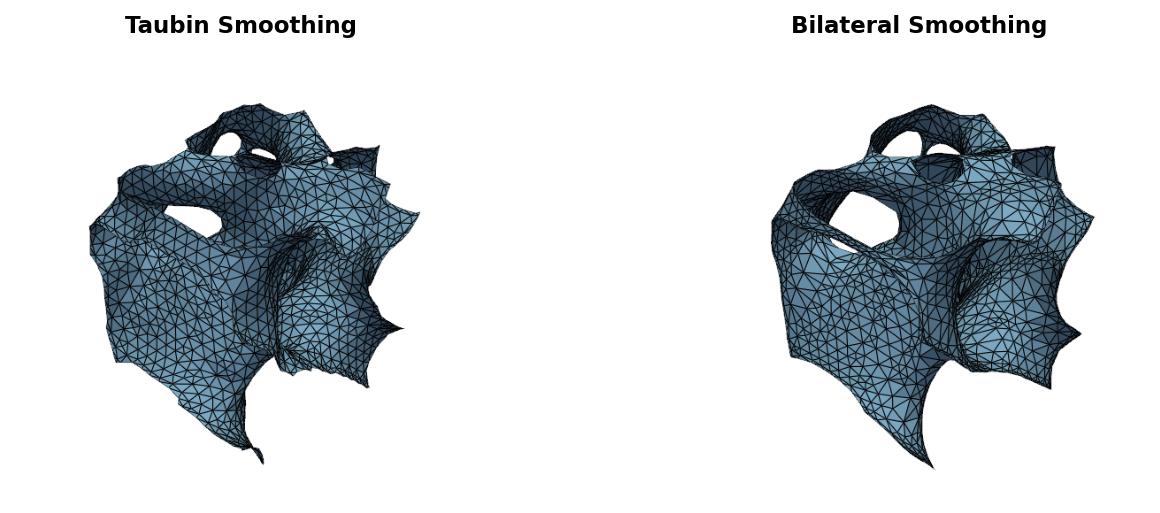
Bilateral filtering weights vertex displacements by normal similarity — neighbors across sharp edges receive near-zero weight, preserving features while smoothing flat regions. See the Parameters guide for tuning sigma values.
CLI usage
Process a field
uv run xtf process field.npy -o output.stlAdd --viz to save a side-by-side comparison plot alongside the mesh:
uv run xtf process field.npy -o output.stl --vizThis saves the mesh to output.stl and a comparison image to output.png.
Visualize without saving a mesh
# Display interactively
uv run xtf viz field.npy

# Save to file
uv run xtf viz field.npy -o comparison.png
Common options
Both process and viz accept these flags:
uv run xtf process input.npy -o output.stl \
    --threshold 0.4 \
    --sigma 1.5 \
    --field-type sdf \
    --direct \
    --field-name xPhys \
--shape 50x100x50| Flag | Description |
|---|---|
--threshold | Field threshold for binarization (default: 0.5) |
--sigma | Gaussian smoothing sigma (default: 1.0) |
--field-type | Input field type: density or sdf (default: density) |
--direct | Skip preprocessing, extract directly from the continuous field |
-f, --field-name | Variable name to extract from multi-field files (.mat, .npz, .vtk, .h5) |
--shape | Reshape flat data to grid, e.g. 100x200 or 10x20x30 (for CSV/TXT) |
Loading from MATLAB
uv run xtf process result.mat -o mesh.stl --field-name xPhysIf --field-name is omitted, the loader auto-detects common design optimization variable names (xPhys, densities, x, rho, dc, density).